Note

This page was generated from user_guide/bfModel/bfModel.ipynb.

The binder version is quite slow due to memory and CPUs limitations

accordingly provided examples have been slightly simplified…

Interactive online version:

Backward forward example

This example will run in approximately 20 minutes.

To run the notebook several post and pre-processing librairies are required:

• panel

• pyvista

• pyevtk

• stripy

To install these dependencies read the documentation in the user guide.

import os
import meshio
import meshplex
import numpy as np
import pandas as pd
import pyvista as pv
import stripy as stripy
from scipy import ndimage
from netCDF4 import Dataset
from scipy.spatial import cKDTree
from scripts import getTecto as tec
from scripts import readOutput as rout
from gospl._fortran import definegtin

In this example we will run a global scale model starting from 15 Millions years ago to present.

For running the experiment, we have the following dataset:

1. a series of paleotopography maps at specific time interval (15 Ma, 5 Ma and 0 Ma) available in the folder data/paleomap as netCDF files.

2. a series of paleoclimate precipitation maps at 5 Ma interval available in the folder data/precipitation as netCDF files.

3. a series of plate velocities at 1 Ma interval available in the folder data/velocity as xy files.

GOAL Using these dataset, we will run a constrained landscape evolution model by using the paleotography maps at available time intervals to force the forward model with tectonic (uplift and subsidence) grids over time.

The example is mainly for illustration purposes. In most cases, the proposed method will require to be tuned over time by modifying the plate reconstructions, the paleotopography / paleoclimate maps and the model input parameters to refine the simulation results over time. Nevertheless, this notebook covers the main principles used during this process.

1. Create gospl input dataset

This first part takes approximately 5 minutes to complete.

1.1. Build gospl mesh

For this example, we will build an icosahedral triangulation using the stripy library. To do so we will define a refinement level of 8 and store the newly created mesh in a folder named input8.

gospl mesh needs the following information:

• nodes coordinates

• cells node indices

• each node neighbours indices

# Refinement level
ref_lvl = 8

# Build the folder in which all gospl input files will be stored
dir_lvl = 'input'+str(ref_lvl)
if not os.path.exists(dir_lvl):
    os.makedirs(dir_lvl)

# Call stripy library
if ref_lvl < 11:
    grid = stripy.spherical_meshes.icosahedral_mesh(include_face_points=False,
                                                    refinement_levels=ref_lvl)
else:
    grid = stripy.spherical_meshes.octahedral_mesh(include_face_points=False,
                                                   refinement_levels=ref_lvl)

str_fmt = "{:25} {:9}"
print(str_fmt.format('Number of points', grid.lpoints))
print(str_fmt.format('Number of cells', grid.simplices.shape[0]))

# Take the unit sphere mesh and assign the Earth radius to the coordinates
radius = 6378137.
coords = np.vstack((grid.points[:,0],grid.points[:,1]))
coords = np.vstack((coords,grid.points[:,2])).T
coords = np.multiply(coords,radius)

# Define mesh cells and nodes neighbourhood
Gmesh = meshplex.MeshTri(coords, grid.simplices)
s = Gmesh.idx_hierarchy.shape
a = np.sort(Gmesh.idx_hierarchy.reshape(s[0], -1).T)
if meshplex.__version__>= "0.14.0":
    Gmesh.edges = {"points": np.unique(a, axis=0)}
    ngbNbs, ngbID = definegtin(len(coords), Gmesh.cells('points'),
                               Gmesh.edges['points'])
else:
    Gmesh.edges = {"nodes": np.unique(a, axis=0)}
    ngbNbs, ngbID = definegtin(len(coords), Gmesh.cells['nodes'],
                               Gmesh.edges['nodes'])

# Create mesh variables
ngbIDs = ngbID[:,:8].astype(int)
vertices = coords.copy()
cells = grid.simplices

# Convert spherical mesh longitudes and latitudes from radian to degree
glat=np.mod(np.degrees(grid.lats)+90, 180.0)
glon=np.mod(np.degrees(grid.lons)+180.0, 360.0)

Number of points             655362
Number of cells             1310720

1.2. Paleo and precipitation maps coordinates

Paleo and precipitation dataset have different resolutions and we first map the newly created mesh coordinates on these two distinct resolutions:

1. coord1 for the paleo-elevation mesh

2. coord2 for the paleo-precipitation mesh

# Paleo-elevation
elevfile = "data/paleomap/0Ma.nc"
data1 = Dataset(elevfile, "r", format="NETCDF4")
img1 = np.fliplr(data1['z'][:,:].T)

# Map mesh coordinates on this dataset
lon1 = img1.shape[0] * glon / 360.0
lat1 = img1.shape[1] * glat / 180.0
coord1 = np.stack((lon1, lat1))
meshlonlat = coord1/10.

# Paleo-precipitation
rainfile = "data/precipitation/0Ma.nc"
data2 = Dataset(rainfile, "r", format="NETCDF4")
img2 = np.fliplr(data2['z'][:,:].T)

# Map mesh coordinates on this dataset
lon2 = img2.shape[0] * glon / 360.0
lat2 = img2.shape[1] * glat / 180.0
coord2 = np.stack((lon2, lat2))

1.3. Interpolation of paleo dataset on gospl mesh

The buildPaleoMesh function below is used to interpolate the paleogrid dataset (elevations and precipitations) on the gospl mesh. It takes the following arguments:

• time: the time interval (here in Ma) to process

• dfolder: the dataset folder containing the paleogrids to interpolate

• outfile: the Numpy file created containing the interpolated values

• coords: the coordinates of the mesh mapped on the dataset resolution

• rain: set to True/False depending of the processed dataset

• visvtk: set to True/False if one want to visualise the output as VTK file

def buildPaleoMesh(time, dfolder, outfile, coord=None, rain=False, visvtk=False, filter=2):

    paleof = dfolder+str(time)+"Ma.nc"
    paleom = outfile+str(time)+"Ma"

    paleodata = Dataset(paleof, "r", format="NETCDF4")

    if rain:
        paleod = paleodata['z'][:,:].T
    else:
        paleod = np.fliplr(paleodata['z'][:,:].T)

    # Apply some smoothing if necessary...
    if filter>0:
        paleod = ndimage.gaussian_filter(paleod,sigma=filter)

    if rain:
        # Interpolate the paleogrid on global mesh
        meshd = ndimage.map_coordinates(paleod, coord, order=2, mode='nearest').astype(np.float64)
        # Conversion from mm/day to m/yr
        meshd *= 365.2422/1000.
        # Save the mesh as compressed numpy file for global simulation
        np.savez_compressed(paleom, r=meshd)
    else:
        # Interpolate the paleogrid on global mesh
        meshd = ndimage.map_coordinates(paleod, coord , order=2, mode='nearest').astype(np.float64)
        # Save the mesh as compressed numpy file for global simulation
        np.savez_compressed(paleom, v=vertices, c=cells, n=ngbIDs.astype(int), z=meshd)

    print("Processing {} to create {} done".format(paleof,paleom+".npz"))

    if visvtk:
        paleovtk = outfile+str(time)+"Ma.vtk"
        if rain:
            vis_mesh = meshio.Mesh(vertices, {'triangle': cells}, point_data={"r":meshd})
        else:
            vis_mesh = meshio.Mesh(vertices, {'triangle': cells}, point_data={"z":meshd})
        meshio.write(paleovtk, vis_mesh)
        print("Writing VTK file {}".format(paleovtk))

    return

# Paleo-elevations
efolder = "data/paleomap/"
efile = dir_lvl+"/elev"
buildPaleoMesh(0, efolder, efile, coord=coord1, rain=False, visvtk=False)
buildPaleoMesh(5, efolder, efile, coord=coord1, rain=False, visvtk=False)
buildPaleoMesh(15, efolder, efile, coord=coord1, rain=False, visvtk=True)

# Paleo-precipitation
rfolder = "data/precipitation/"
rfile = dir_lvl+"/rain"
buildPaleoMesh(0, rfolder, rfile, coord=coord2, rain=True, visvtk=False)
buildPaleoMesh(5, rfolder, rfile, coord=coord2, rain=True, visvtk=False)
buildPaleoMesh(10, rfolder, rfile, coord=coord2, rain=True, visvtk=False)
buildPaleoMesh(15, rfolder, rfile, coord=coord2, rain=True, visvtk=False)


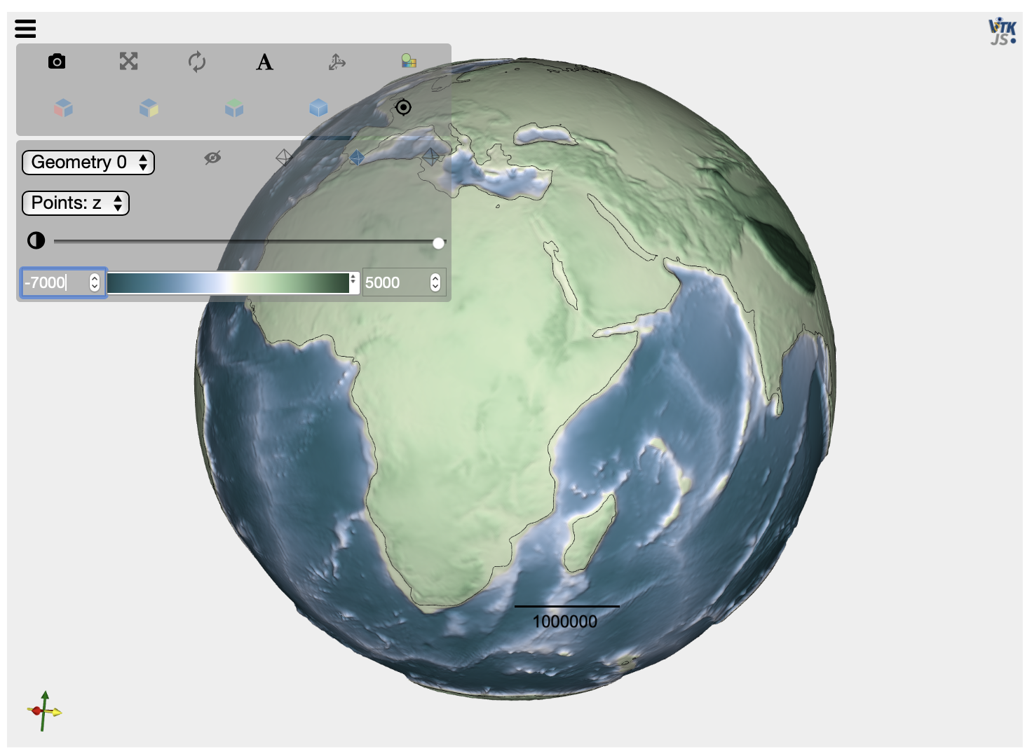
# Check the mesh validity by loading the created VTK file
mesh = pv.read('input8/elev15Ma.vtk')
elev = mesh.get_array(name='z')
scale = 20.
factor = 1.+ (elev/radius)*scale
mesh.points[:, 0] *= factor
mesh.points[:, 1] *= factor
mesh.points[:, 2] *= factor
contour = mesh.contour([0])
plot = pv.PlotterITK()
plot.add_mesh(mesh, scalars="z")
plot.add_mesh(contour, color="black", opacity=1.)
plot.show()

Processing data/paleomap/0Ma.nc to create input8/elev0Ma.npz done
Processing data/paleomap/5Ma.nc to create input8/elev5Ma.npz done
Processing data/paleomap/15Ma.nc to create input8/elev15Ma.npz done
Writing VTK file input8/elev15Ma.vtk
Processing data/precipitation/0Ma.nc to create input8/rain0Ma.npz done
Processing data/precipitation/5Ma.nc to create input8/rain5Ma.npz done
Processing data/precipitation/10Ma.nc to create input8/rain10Ma.npz done
Processing data/precipitation/15Ma.nc to create input8/rain15Ma.npz done

1.4. Velocity fields on gospl mesh

We will now read the paleo-displacement grids stored in the data/velocity as xy files.

These velocities have been obtained from the gPlates web protal (in cm/yr) and have a specific format, we will use pandas library to parse these files.

To get X,Y,Z velocities on gospl mesh, we will define a kdTree using ScipPy spatial cKDTree function and for simplicity we will use the closest point indice to assign the velocity on each node of the triangulation.

First we build the tree and find the closest indices:

# Open the 3D displacement maps (xy files) and store it as a pandas dataframe
dir_vel = 'data/velocity'
gPlates = dir_vel+'/velocity_0.00Ma.xy'
data = pd.read_csv(gPlates, sep=r'\s+', engine='c',
                   header=None, skiprows=[0,1,2,3,4,5,65166],
                   error_bad_lines=True, na_filter=False,
                   dtype=np.float64, low_memory=False)

vlon = data.values[:,0]+180.
vlat = data.values[:,1]+90.

# Build the kdtree
tree = cKDTree(list(zip(vlon, vlat)))
dist, closeID = tree.query(list(zip(meshlonlat[0,:], meshlonlat[1,:])), k = 1)

We will then call the nearestPaleoDisp function below to build the displacement files induced by the moving plates required by gospl.

This function takes the following arguments:

• gPlates: the input velocity file name

• outfile: the Numpy file created containing the interpolated velocity values

• dfolder: the dataset folder containing the paleogrids to interpolate

• reverse: set to True/False depending of the type of model that is ran either backward (True) or forward (False)

• visvtk: set to True/False if one want to visualise the output as VTK file

def nearestPaleoDisp(gPlates=None, outfile=None, reverse=False, visvtk=False):
    '''
    Reading paleo-displacement grids
    '''

    # Open gPlates 1 degree 3D displacement maps (xy files)
    data = pd.read_csv(gPlates, sep=r'\s+', engine='c', header=None, skiprows=[0,1,2,3,4,5,65166],
                       error_bad_lines=True, na_filter=False, dtype=np.float64, low_memory=False)

    # Conversion from cm/yr to m/yr
    if reverse:
        tmpx = -data.values[:,2]/100.
        tmpy = -data.values[:,3]/100.
        tmpz = -data.values[:,4]/100.
    else:
        tmpx = data.values[:,2]/100.
        tmpy = data.values[:,3]/100.
        tmpz = data.values[:,4]/100.

    # Interpolate the paleo displacement on global mesh
    dX = tmpx.flatten()[closeID].reshape(meshlonlat[0,:].shape)
    dY = tmpy.flatten()[closeID].reshape(meshlonlat[0,:].shape)
    dZ = tmpz.flatten()[closeID].reshape(meshlonlat[0,:].shape)

    disps = np.stack((dX, dY, dZ)).T

    # Save the mesh as compressed numpy file for global simulation
    np.savez_compressed(outfile, xyz=disps)

    if visvtk:
        vis_mesh = meshio.Mesh(vertices, {'triangle': cells}, point_data={"ux":dX,"uy":dY,"uz":dZ})
        meshio.write(outfile+".vtk", vis_mesh)
        print("Writing VTK file {}".format(outfile+".vtk"))

    print("Processing {} to create {}".format(gPlates,outfile+".npz"))

    return

In this example, we will apply the function over a 1 Ma increment for both backward and forward models. The function will create displacement file at the same temporal resolution (1 Ma) with 3D displacements in m/yr corresponding to the plate velocities.

# Specify most recent time in Ma
startMa = 0
# Specify deepest time in Ma
endMa = 15
# Specify paleodisp interval
dtMa = 1

timeframe = np.arange(startMa,endMa+dtMa,dtMa)

p = timeframe[0]
for k in range(len(timeframe)):
    f_gplates = dir_vel+'/velocity_'+str(k+p)+'.00Ma.xy'
    paleo_disp = dir_lvl+'/disp'+str(k+p)+'Ma'
    paleo_backdisp = dir_lvl+'/backdisp'+str(k+p)+'Ma'
    nearestPaleoDisp(gPlates=f_gplates, outfile=paleo_disp, reverse=False, visvtk=False)
    nearestPaleoDisp(gPlates=f_gplates, outfile=paleo_backdisp, reverse=True, visvtk=False)

Processing data/velocity/velocity_0.00Ma.xy to create input8/disp0Ma.npz
Processing data/velocity/velocity_0.00Ma.xy to create input8/backdisp0Ma.npz
Processing data/velocity/velocity_1.00Ma.xy to create input8/disp1Ma.npz
Processing data/velocity/velocity_1.00Ma.xy to create input8/backdisp1Ma.npz
Processing data/velocity/velocity_2.00Ma.xy to create input8/disp2Ma.npz
Processing data/velocity/velocity_2.00Ma.xy to create input8/backdisp2Ma.npz
Processing data/velocity/velocity_3.00Ma.xy to create input8/disp3Ma.npz
Processing data/velocity/velocity_3.00Ma.xy to create input8/backdisp3Ma.npz
Processing data/velocity/velocity_4.00Ma.xy to create input8/disp4Ma.npz
Processing data/velocity/velocity_4.00Ma.xy to create input8/backdisp4Ma.npz
Processing data/velocity/velocity_5.00Ma.xy to create input8/disp5Ma.npz
Processing data/velocity/velocity_5.00Ma.xy to create input8/backdisp5Ma.npz
Processing data/velocity/velocity_6.00Ma.xy to create input8/disp6Ma.npz
Processing data/velocity/velocity_6.00Ma.xy to create input8/backdisp6Ma.npz
Processing data/velocity/velocity_7.00Ma.xy to create input8/disp7Ma.npz
Processing data/velocity/velocity_7.00Ma.xy to create input8/backdisp7Ma.npz
Processing data/velocity/velocity_8.00Ma.xy to create input8/disp8Ma.npz
Processing data/velocity/velocity_8.00Ma.xy to create input8/backdisp8Ma.npz
Processing data/velocity/velocity_9.00Ma.xy to create input8/disp9Ma.npz
Processing data/velocity/velocity_9.00Ma.xy to create input8/backdisp9Ma.npz
Processing data/velocity/velocity_10.00Ma.xy to create input8/disp10Ma.npz
Processing data/velocity/velocity_10.00Ma.xy to create input8/backdisp10Ma.npz
Processing data/velocity/velocity_11.00Ma.xy to create input8/disp11Ma.npz
Processing data/velocity/velocity_11.00Ma.xy to create input8/backdisp11Ma.npz
Processing data/velocity/velocity_12.00Ma.xy to create input8/disp12Ma.npz
Processing data/velocity/velocity_12.00Ma.xy to create input8/backdisp12Ma.npz
Processing data/velocity/velocity_13.00Ma.xy to create input8/disp13Ma.npz
Processing data/velocity/velocity_13.00Ma.xy to create input8/backdisp13Ma.npz
Processing data/velocity/velocity_14.00Ma.xy to create input8/disp14Ma.npz
Processing data/velocity/velocity_14.00Ma.xy to create input8/backdisp14Ma.npz
Processing data/velocity/velocity_15.00Ma.xy to create input8/disp15Ma.npz
Processing data/velocity/velocity_15.00Ma.xy to create input8/backdisp15Ma.npz

2. Run gospl

This step takes about 10 minutes to complete.

Running gospl is done by calling the runBF.py script.

The Python script will do the following:

1. run the backward models (using the backward15Ma.yml and backward10Ma.yml input files). The backward models do not have surface processes activated and only the backward displacements computed above are used to move the elevation over time.

2. combine each backward model outputs together using the scripts/mergeBack.py file.

3. run the forward model (using the forward.yml input file). This model accounts for climatic forcing, tectonic forcing and surface processes. Also it will for each 1 million year interval compute the differences between the simulated elevation and the backward ones and apply a scaling factor to force the elevations to approach the paleo-elevations at 5 and 15 Ma. The computed scaled differences are reapplied at the previous time step as a vertical tectonic map.

You can open the input files to look at the parameters that are setup for this example. A complete list of the gospl input variables is available in the user guide documentation.

---

A series of 3 input files are provided and can be used to run backward and forward models. The 2 backward models are divided in steps:

1. :code:backward15Ma.yml runs from 15 Ma to 10 Ma in model time but corresponds in real time in a backward model starting at 0 Ma and running back to 5 Ma ago;

2. :code:backward10Ma.yml goes from 10 Ma to 0 Ma in model time, i.e. 5 Ma ago to 15 Ma ago in real time.

When looking at these input files pay attention at the order of the tectonic meshes that force the model. It is also worth mentioning that for these backward models we do not compute the surface processes as a result we set :code:fast and :code:backward to True.

# On a single processor...
#%run runBF.py

# In parallel...
!mpirun -np 4 python3 runBF.py

--- Initialisation Phase (14.72 seconds)
+++ Output Simulation Time: -15000000.00 years
--- Computational Step                       (0.55 seconds)
+++ Output Simulation Time: -14000000.00 years
--- Computational Step                       (0.86 seconds)
+++ Output Simulation Time: -13000000.00 years
--- Computational Step                       (0.85 seconds)
+++ Output Simulation Time: -12000000.00 years
--- Computational Step                       (0.86 seconds)
+++ Output Simulation Time: -11000000.00 years
--- Computational Step                       (0.86 seconds)
+++ Output Simulation Time: -10000000.00 years
--- Computational Step                       (0.29 seconds)

+++
+++ Total run time (19.03 seconds)
+++

--- Initialisation Phase (14.40 seconds)
+++ Output Simulation Time: -10000000.00 years
--- Computational Step                       (0.51 seconds)
+++ Output Simulation Time: -9000000.00 years
--- Computational Step                       (0.84 seconds)
+++ Output Simulation Time: -8000000.00 years
--- Computational Step                       (0.79 seconds)
+++ Output Simulation Time: -7000000.00 years
--- Computational Step                       (0.83 seconds)
+++ Output Simulation Time: -6000000.00 years
--- Computational Step                       (0.83 seconds)
+++ Output Simulation Time: -5000000.00 years
--- Computational Step                       (0.83 seconds)
+++ Output Simulation Time: -4000000.00 years
--- Computational Step                       (0.81 seconds)
+++ Output Simulation Time: -3000000.00 years
--- Computational Step                       (0.80 seconds)
+++ Output Simulation Time: -2000000.00 years
--- Computational Step                       (0.85 seconds)
+++ Output Simulation Time: -1000000.00 years
--- Computational Step                       (0.81 seconds)
+++ Output Simulation Time: 0.00 years
--- Computational Step                       (0.26 seconds)

+++
+++ Total run time (22.60 seconds)
+++

Read each input files done...
Create output directory and save XDMF file...
Save XMF files...
Merging models done...

--- Initialisation Phase (16.73 seconds)
+++ Output Simulation Time: -15000000.00 years
--- Computational Step                       (10.99 seconds)
+++ Output Simulation Time: -14000000.00 years
--- Computational Step                       (11.36 seconds)
+++ Output Simulation Time: -14000000.00 years
--- Computational Step                       (10.17 seconds)
+++ Output Simulation Time: -13000000.00 years
--- Computational Step                       (10.97 seconds)
+++ Output Simulation Time: -13000000.00 years
--- Computational Step                       (10.76 seconds)
+++ Output Simulation Time: -12000000.00 years
--- Computational Step                       (11.27 seconds)
+++ Output Simulation Time: -12000000.00 years
--- Computational Step                       (11.80 seconds)
+++ Output Simulation Time: -11000000.00 years
--- Computational Step                       (11.57 seconds)
+++ Output Simulation Time: -11000000.00 years
--- Computational Step                       (12.26 seconds)
+++ Output Simulation Time: -10000000.00 years
--- Computational Step                       (12.35 seconds)
+++ Output Simulation Time: -10000000.00 years
--- Computational Step                       (13.12 seconds)
+++ Output Simulation Time: -9000000.00 years
--- Computational Step                       (13.01 seconds)
+++ Output Simulation Time: -9000000.00 years
--- Computational Step                       (12.94 seconds)
+++ Output Simulation Time: -8000000.00 years
--- Computational Step                       (13.58 seconds)
+++ Output Simulation Time: -8000000.00 years
--- Computational Step                       (13.71 seconds)
+++ Output Simulation Time: -7000000.00 years
--- Computational Step                       (15.08 seconds)
+++ Output Simulation Time: -7000000.00 years
--- Computational Step                       (15.06 seconds)
+++ Output Simulation Time: -6000000.00 years
--- Computational Step                       (14.83 seconds)
+++ Output Simulation Time: -6000000.00 years
--- Computational Step                       (14.85 seconds)
+++ Output Simulation Time: -5000000.00 years
--- Computational Step                       (13.31 seconds)
+++ Output Simulation Time: -5000000.00 years
--- Computational Step                       (14.03 seconds)
+++ Output Simulation Time: -4000000.00 years
--- Computational Step                       (13.66 seconds)
+++ Output Simulation Time: -4000000.00 years
--- Computational Step                       (16.58 seconds)
+++ Output Simulation Time: -3000000.00 years
--- Computational Step                       (16.04 seconds)
+++ Output Simulation Time: -3000000.00 years
--- Computational Step                       (20.30 seconds)
+++ Output Simulation Time: -2000000.00 years
--- Computational Step                       (18.10 seconds)
+++ Output Simulation Time: -2000000.00 years
--- Computational Step                       (17.72 seconds)
+++ Output Simulation Time: -1000000.00 years
--- Computational Step                       (16.41 seconds)
+++ Output Simulation Time: -1000000.00 years
--- Computational Step                       (14.99 seconds)
+++ Output Simulation Time: 0.00 years
--- Computational Step                       (14.89 seconds)
+++ Output Simulation Time: 0.00 years
--- Computational Step                       (12.47 seconds)

+++
+++ Total run time (444.97 seconds)
+++

3. Visualisation in a notebook environment

The preferred way for visualising the model output is via Paraview by loading the time series file called gospl.xdmf available in the output folder (here called forward). A Paraview file is also provided: pvstate.pvsm. It can be loaded as a state in Paraview and should work once the relative path of the gospl.xdmf file has been correctly defined to match with your local repository structure.

Amongst the temporal variables outputed by gospl you will find:

• surface elevation elev.

• cumulative erosion & deposition values erodep.

• flow accumulation flowAcc before pit filling.

• flow accumulation fillAcc for depressionless surface.

• river sediment load sedLoad.

• fine sediment load sedLoadf when dual lithologies are accounted for.

• uplift subsidence values if vertical tectonic forcing is considered uplift.

• horizontal displacement values when considered hdisp.

• precipitation maps based on forcing conditions rain.

Several filters, rendering and calculation can be done with Paraview but are beyond the scope of this example.

Here you will use the readOutput.py functions available in the scripts folder to visualise directly the model output in the notebook at the final time step.

The function requires several arguments:

• filename: the name of the input file

• step: the step you wish to output (here set to 15 corresponding to the last output based on the input parameters: start time 15 Ma, end time present with an output every 1 million year)

# Reading the final output generated by gospl
output = rout.readOutput(filename='forward.yml',step=15)

# Exporting the final output as a VTK mesh
output.exportVTK('step15.vtk')

Writing VTK file step15.vtk

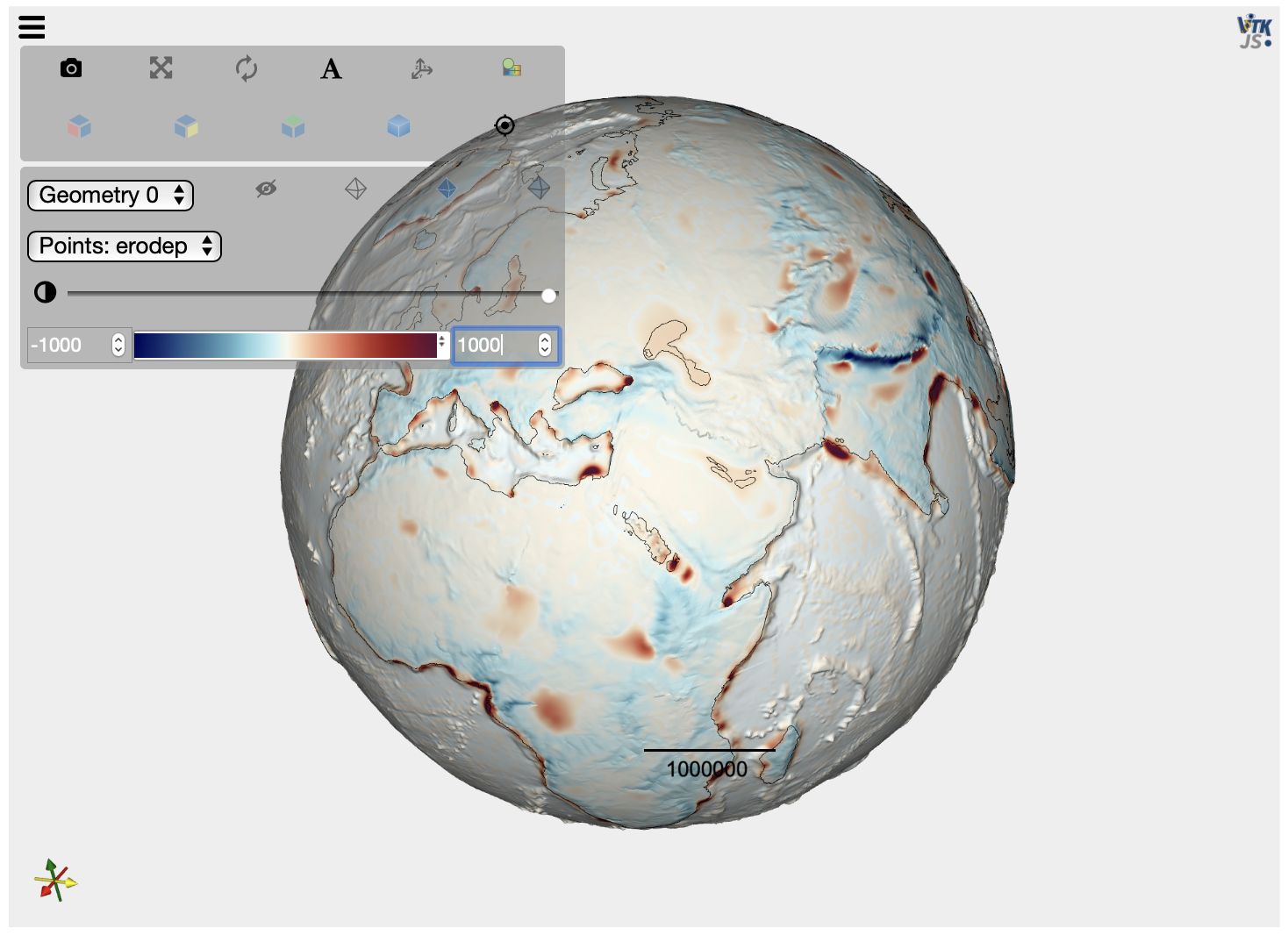
We can now visualise the VTK output in the notebook directly:

mesh = pv.read('step15.vtk')
elev = mesh.get_array(name='elev')

earthRadius = 6.371e6
scale = 20.
factor = 1.+ (elev/earthRadius)*scale

mesh.points[:, 0] *= factor
mesh.points[:, 1] *= factor
mesh.points[:, 2] *= factor

contour = mesh.contour([0])

plot = pv.PlotterITK()
plot.add_mesh(mesh, scalars="elev")
plot.add_mesh(contour, color="black", opacity=1.)
plot.show()

4. Export vertical displacements

Here, we illustrate how we can extract some of gospl output variables using some Python functions.

As an example, the scripts/getTecto.py function can export the computed vertical tectonic rates (uplift and subsidence) obtained from the backward/forward model and create vertical tectonic input files (input8/vdispXMa.npz) that can be directly applied to the forward model without having to run it in backward/forward mode.

# Initialise the tectonic class
tect = tec.getTecto(filename='forward.yml')

# Define simulation time intervals in Ma
startMa = 0
endMa = 15

# Specify paleodisp interval
dtMa = 1
timeframe = np.arange(startMa,endMa+dtMa,dtMa)
timeframe = np.flip(timeframe)

# Create the vertical tectonic input files over time
tect.readData(out=dir_lvl+'/vdisp',time=timeframe)

Read uplift/subsidence for step: 1
Read uplift/subsidence for step: 2
Read uplift/subsidence for step: 3
Read uplift/subsidence for step: 4
Read uplift/subsidence for step: 5
Read uplift/subsidence for step: 6
Read uplift/subsidence for step: 7
Read uplift/subsidence for step: 8
Read uplift/subsidence for step: 9
Read uplift/subsidence for step: 10
Read uplift/subsidence for step: 11
Read uplift/subsidence for step: 12
Read uplift/subsidence for step: 13
Read uplift/subsidence for step: 14
Read uplift/subsidence for step: 15

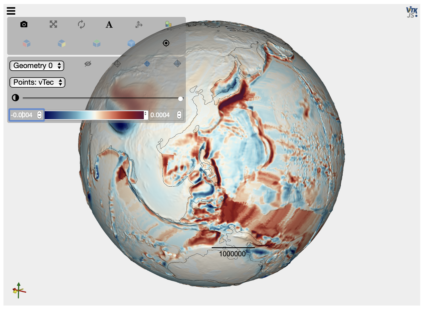
We can check one of the tectonic input file values by creating a VTK file and plotting it in the Jupyter notebook…

checkvtk = dir_lvl+'/vtec15Ma.vtk'
etopofile = dir_lvl+'/elev15Ma.npz'
topo = np.load(etopofile)
elev = topo['z']

vdispfile = dir_lvl+'/vdisp15Ma.npz'
data = np.load(vdispfile)
vdisp = data['z']

vis_mesh = meshio.Mesh(vertices, {'triangle': cells}, point_data={"Z":elev, "vTec":vdisp})
meshio.write(checkvtk, vis_mesh)

print("Writing VTK file {}".format(checkvtk))

# Plot the tectonic vertical forcing by loading the created VTK file
mesh = pv.read(checkvtk)
elev = mesh.get_array(name='Z')
scale = 20.
factor = 1.+ (elev/radius)*scale
mesh.points[:, 0] *= factor
mesh.points[:, 1] *= factor
mesh.points[:, 2] *= factor
contour = mesh.contour([0])
plot = pv.PlotterITK()
plot.add_mesh(mesh, scalars="vTec")
plot.add_mesh(contour, color="black", opacity=1.)
plot.show()

Writing VTK file input8/vtec15Ma.vtk

previous

Input file parameters

next

100 Ma backward forward model