HPC scaling & performance

This page reports honest strong-scaling measurements for goSPL on production, global-scale meshes. “Strong scaling” means the same problem is solved on an increasing number of MPI ranks (cores): ideally the wall-clock time halves when the core count doubles. We report both the speedup and the parallel efficiency, and we are explicit about where — and why — efficiency falls away.

All runs exercise the full model (flow accumulation, river incision/deposition, continental and marine sediment routing, hillslope diffusion, flexural isostasy, tectonic forcing) so the numbers reflect a realistic workload, not a single kernel.

Fig. 8 Example goSPL output on the 10 km global mesh (5.9 M nodes) used for the scaling benchmarks below — the full landscape-evolution workload (drainage, erosion/deposition, sediment routing) that each timed step solves.

Global mesh resolutions

The benchmarks use three icosahedral-derived global meshes (variable resolution; the edge lengths below are in km):

Cell width (km)	Nodes	Faces	Edge min (km)	Edge max (km)	Edge mean (km)
5	23,655,606	47,311,208	3.73	6.78	4.99
8	9,246,354	18,492,704	6.11	10.96	7.98
10	5,916,934	11,833,864	7.59	13.61	9.98

How the benchmark is run

• Hardware: NCI Gadi (48-core nodes; counts above 48 span whole nodes). The harness lives in scripts/scaling/ (see its README.md); each rank count is a separate, optionally chained job (submit_sweep.sh → gadi.pbs).

• What is timed: a fixed number of model steps with the wall-clock phase profiler enabled and I/O disabled (--io off), so the numbers reflect compute + communication, not HDF5 bandwidth.

• Baseline: a global mesh is memory-infeasible at very low core counts (the 10 km mesh needs ~6.6 GB on the heaviest rank and cannot start below ~16 ranks; finer meshes need more). There is therefore no 1-CPU run to normalise against. We follow the standard convention and baseline to the smallest feasible rank count \(p_0\) in each sweep:

  \[S(p) = \frac{T(p_0)}{T(p)}, \qquad E(p) = S(p)\,\frac{p_0}{p}, \qquad \text{ideal: } S = p/p_0,\ E = 1.\]

  When reading the figure, the dashed line is the ideal \(p/p_0\), and efficiency 1.0 is perfect scaling relative to \(p_0\) — not to a single core.

Results

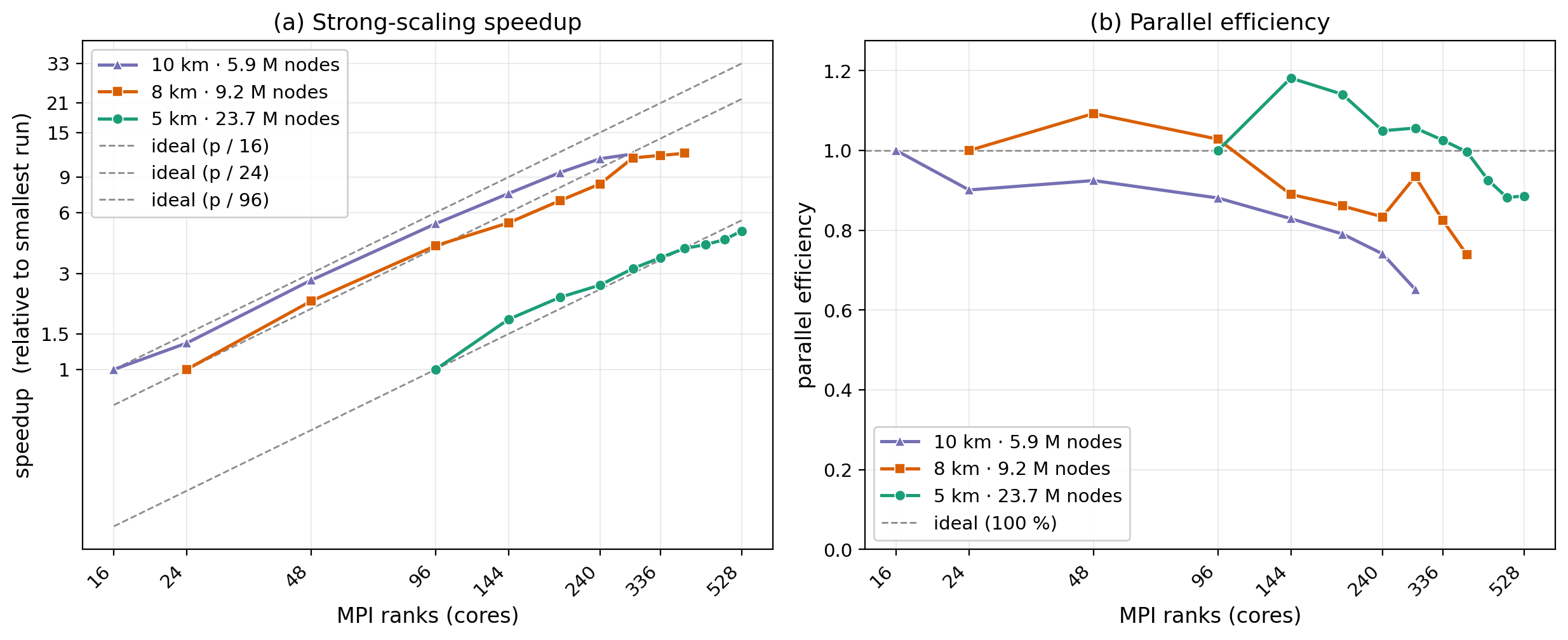
Fig. 9 Strong-scaling speedup (a) and parallel efficiency (b) versus MPI rank count, for the three global meshes above. Markers are measured points; dashed lines are the ideal (each sweep is baselined to its own smallest feasible rank count — 16, 24 and 96 for the 10, 8 and 5 km meshes — so the three curves have different ideal references).

10 km mesh (5.9 M nodes), baseline = 16 ranks:

Ranks	Wall (s)	Speedup	Efficiency	RSS / rank (GB)
16	521.3	1.00	1.00	6.6
24	385.6	1.35	0.90	6.6
48	187.9	2.77	0.92	6.6
96	98.6	5.29	0.88	6.6
144	69.9	7.46	0.83	6.7
192	54.9	9.49	0.79	6.6
240	46.9	11.11	0.74	6.6
288	44.4	11.73	0.65	6.6

8 km mesh (9.2 M nodes), baseline = 24 ranks:

Ranks	Wall (s)	Speedup	Efficiency	RSS / rank (GB)
24	800.7	1.00	1.00	9.9
48	366.4	2.19	1.09	9.7
96	194.7	4.11	1.03	9.8
144	150.0	5.34	0.89	9.8
192	116.3	6.89	0.86	9.8
240	96.0	8.34	0.83	9.8
288	71.4	11.22	0.93	9.8
336	69.4	11.54	0.82	10.0
384	67.7	11.82	0.74	10.0

5 km mesh (23.7 M nodes), baseline = 96 ranks:

Ranks	Wall (s)	Speedup	Efficiency	RSS / rank (GB)
96	766.6	1.00	1.00	24.2
144	432.5	1.77	1.18	24.3
192	336.0	2.28	1.14	24.4
240	292.2	2.62	1.05	24.4
288	241.9	3.17	1.06	24.3
336	213.6	3.59	1.03	24.3
384	192.3	3.99	1.00	24.3
432	184.0	4.17	0.93	24.3
480	173.8	4.41	0.88	24.3
528	157.3	4.87	0.89	24.2

Reading the results

• Near-ideal to ~100 ranks. Efficiency holds around 0.88–0.92 out to 96 ranks (a 5.3× speedup), i.e. the compute-heavy phases — sediment routing (sed), marine deposition (sea), flow accumulation, erosion — all parallelise well and are perfectly load-balanced (per-phase imbalance ≈ 1.00).

• Gentle decline beyond that, by Amdahl’s law. Efficiency eases to 0.74 at 240 ranks and 0.65 at 288. This is not a load-balance problem; it is the growing weight of the small serial sections as the parallel work shrinks:

  • flexure (global spherical-harmonic solve, pyshtools) is a flat ~4 s floor at every rank count — genuinely serial;

  • pit filling parallelises partway (the local priority-flood fill scales — 10 km: ~16 → ~8 s) then flattens toward the floor set by its serial, rank-0 spillover-graph master solve (whose cost tracks the partition perimeter and so creeps up slightly with rank count).

  Together these set the practical ceiling (see Where the time goes below).

• Each mesh has a useful core ceiling that rises with size. For 10 km the practical sweet spot is ≈ 240 ranks (11.1× at 74 %); past 288 it’s just serial floors. The 8 km mesh plateaus by ~288–384: 288 → 336 → 384 gains only ~5 % wall-clock in total (71.4 → 69.4 → 67.7 s) while efficiency falls 0.93 → 0.82 → 0.74, so ~288 cores is its practical limit. The 5 km mesh, with far more parallel work, keeps paying off much further — still improving at 528 ranks (4.87× speedup), though efficiency eases from ~1.0 (≤ 384) to ~0.89 (528). The larger the mesh, the more cores it can use before the serial floors (flexure, pit-graph) dominate.

• Memory is the lower bound, not a per-rank growth. Peak RSS on the heaviest rank stays flat with rank count — ~6.6 GB (10 km) / ~9.9 GB (8 km) / ~24 GB (5 km) — because the dominant arrays are replicated, mesh-sized (mpoints) globals that do not decompose. That flat floor is what sets the smallest feasible rank count, which rises with mesh size: 16 ranks at 10 km, 24 at 8 km, 96 at 5 km. At 5 km the peak is concentrated on rank 0 (which holds the serial pit-spillover graph): the max-rank RSS is ~24 GB while the per-rank average (rss_sum / ranks) is only ~3 GB, so the run still fits on standard nodes even though the headline number looks large. (A 48-rank 5 km run — everything on a single 192 GB node — is OOM-killed on rank 0 (SIGKILL); PBS recorded ~180 GB, which undercounts the transient peak that tripped the node limit — the sampled figure lags the actual peak, and a “192 GB” node leaves only ~185 GB to the job after OS overhead. Spread over two nodes, 96 ranks fits — which is why 96 is the smallest feasible 5 km count.)

• The 8 km and 5 km meshes scale superlinearly at intermediate rank counts (8 km: efficiency 1.09 at 48, 1.03 at 96; 5 km: 1.18 at 144, 1.14 at 192 — above the ideal line). This is genuine, not a measurement artefact: at the baseline the per-rank working set is large and spills cache / saturates memory bandwidth, so the baseline is slow; adding ranks shrinks each rank’s slice until it fits, and per-core throughput rises. The effect fades once the slices are cache-resident, after which the usual Amdahl decline takes over (8 km: 0.89 → 0.83 to 240; 10 km, with its small per-rank slice already cache-resident at the 16-rank baseline, shows no super-linearity and declines from the start). We report efficiency uncapped — super-linear points are shown as measured, not clipped to 1.0.

Note

Efficiency is reported relative to each mesh’s smallest feasible run (\(p_0\) = 16 ranks at 10 km, 24 at 8 km, 96 at 5 km), not a single core. We deliberately do not extrapolate a virtual 1-core time to inflate the speedup. One consequence: because the baseline itself is memory-bandwidth bound, efficiency can legitimately exceed 1.0 at intermediate rank counts (see the 8 km mesh) — a real super-linear effect we leave un-clipped rather than hide.

Where the time goes

Splitting the wall-clock by phase shows why the curves bend, and it’s the honest way to see what scales and what doesn’t.

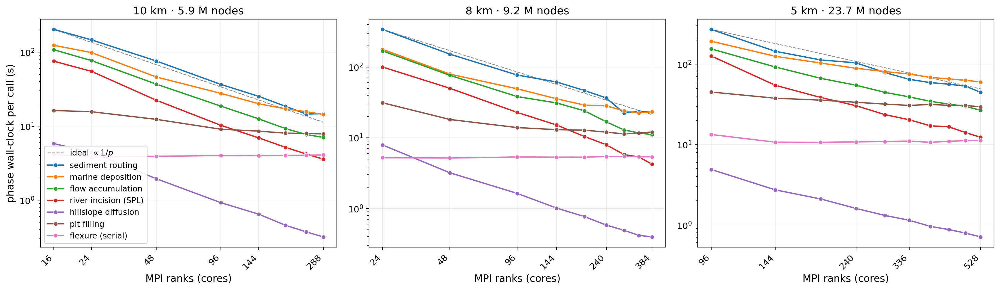
Fig. 10 Mean per-call wall-clock of the main model phases versus rank count, one panel per mesh (log–log; the dashed line is the ideal \(\propto 1/p\)). Only top-level phases are shown — the flow_* sub-phases nest inside flow accumulation — with flexure (the serial floor) and pit filling (partly serial) broken out.

• The compute phases scale well. Sediment routing, marine deposition, flow accumulation, river incision (SPL) and hillslope diffusion all track the \(1/p\) ideal across the whole range — they dominate the budget and are what makes the overall speedup hold up.

• Flexure is the one genuinely serial floor. The global spherical-harmonic load solve is essentially flat with rank count (it does not decompose), so as the parallel phases shrink it becomes a larger fraction — the main Amdahl term behind the efficiency decline.

• Pit filling is only *partly* serial. It does scale down at first (10 km: ~16 → ~8 s) — the local priority-flood fill is parallel — but it flattens toward a floor set by its rank-0 spillover-graph master solve (whose own cost even creeps up slightly with rank count, tracking the partition perimeter). So it scales partway and then plateaus, rather than being a fixed cost like flexure.

• The floors grow with mesh size. Flexure rises ~4 → ~5 → ~11 s and pit filling’s baseline ~16 → ~32 → ~45 s from the 10 → 8 → 5 km meshes, so on finer meshes the serial fraction sets in at a (proportionally) lower rank count — the motivation for keeping these two phases on the optimisation radar.

Reproducing

The summary CSVs and the figure script live in docs/user_guide/scaling/. To regenerate both figures (scaling_hpc.png and scaling_phases.png) after adding or updating a sweep CSV (scaling_<N>km.csv):

python docs/user_guide/scaling/make_scaling_figure.py

The script auto-discovers every scaling_<N>km.csv in that folder, so a new resolution is picked up by dropping its CSV in and re-running. To run a sweep and produce a CSV, see scripts/scaling/README.md (the submit_sweep.sh → analyze_scaling.py → plot_scaling.py workflow).